Time Series Intro
Applications of Data Science - Class 20
Giora Simchoni
Stat. and OR Department, TAU
2023-04-07
What is a Time Series?
A time series is a sequence of observations taken sequentially in time.
Code
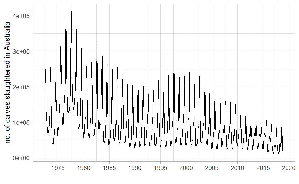
library (tidyverse)library (tsibble)library (tsibbledata)library (feasts)|> filter (Animal == "Calves" ) |> index_by () |> summarise (Count = sum (Count)) |> autoplot (log (Count)) + labs (x = "" , y = "log no. of calves slaughtered in Australia" ) + scale_x_yearmonth (date_breaks = "5 year" , date_labels = "%Y" ) + theme_light ()
TSA Focuses on:
Discrete measurements
Equally-spaced
Usually no missing values
Not that short (say > 20? 50?)
Time is intrinsic, it is not just another feature
Could involve time-varying/non-time-varying explaining features
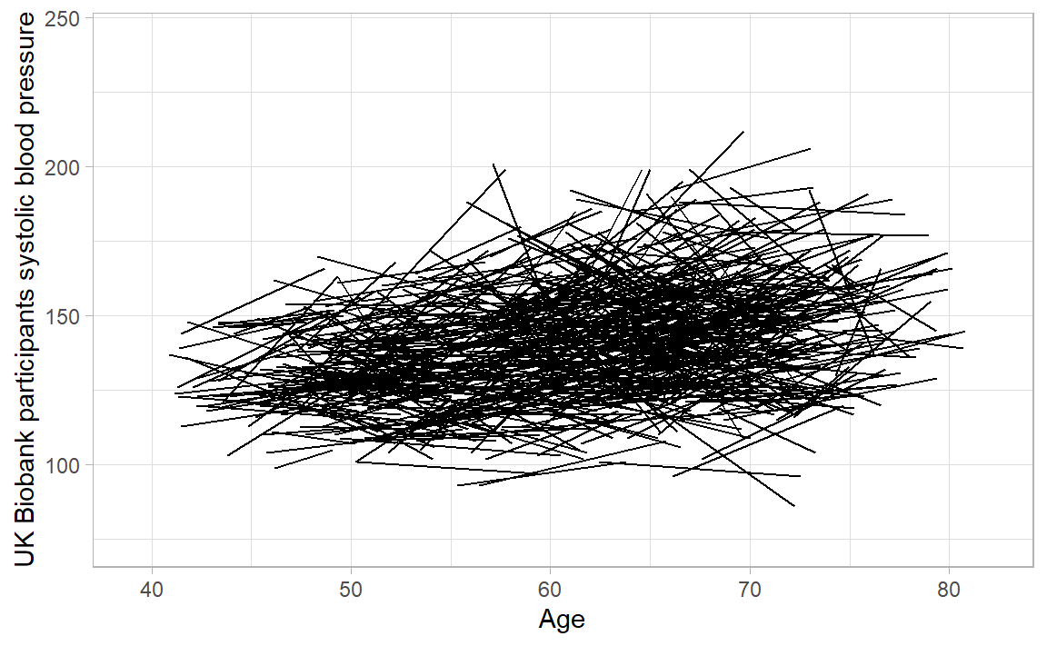
E.g. this is more of a longitudinal/growth-curve/cohort dataset:
TSA Goals
Forecasting (prediction)
Monitoring: outlier detection, alert systems
Describing: the TS dynamics, input features contribution
Planning: control schemes, intervention analyses, sensitivity analyses
Clustering: with multivariate TS
The Date class
<- as.Date ("1915-6-16" )class (date_obj)
Internally, Date objects are stored as the number of days since January 1, 1970, using negative numbers for earlier dates.
So this naturally works:
[1] "1915-06-16" "1915-06-26"
Can also accept different formats and has a few built-in functions:
<- as.Date ("1/15/2001" ,format= "%m/%d/%Y" )months (date_obj)
The POSIX classes
POSIX is a slightly more evolved class from UNIX, holding number of seconds since January 1, 1970, and a time zone may be specified:
[1] "2023-04-07 14:04:13 IDT"
The POSIXlt class will store time in a list with useful elements:
<- as.POSIXlt (now, tz = "GMT" )$ hour
The lubridate package
Parsing dates:
Making dates:
make_date (year = 2013 , month = 2 , day = 12 )
Converting between formats:
Getting components:
<- ymd_hms ("2016-07-08 12:34:56" )year (datetime)
Duration, time maths:
today () - ymd ("2020-01-01" ) #base R difftime object
Time difference of 1192 days
as.duration (today () - ymd ("2020-01-01" ))
[1] "102988800s (~3.26 years)"
[1] "2022-04-06 18:00:00 UTC"
The Tidyverts
A suite of packages for TSA, the tidy way, led by Rob J. Hyndman :
tsibble: The data.frametibble re-imagined for temporal datatsibbledata: TS datasetsfeasts: Feature extraction for TS + Some useful gg plotsfable and fabletools: The modeling and forecasting packagemore and more to come.
See tidyverts.org .
tsibbleNeed a time index:
library (tsibble)tsibble (date = as.Date ("2017-01-01" ) + 0 : 9 ,value = rnorm (10 )
# A tsibble: 10 x 2 [1D]
   date        value
   <date>      <dbl>
 1 2017-01-01  1.60
 2 2017-01-02  1.07
 3 2017-01-03 -0.329
 4 2017-01-04 -0.753
 5 2017-01-05 -1.28
 6 2017-01-06 -0.285
 7 2017-01-07  0.289
 8 2017-01-08 -0.342
 9 2017-01-09 -0.720
10 2017-01-10  0.696
Here, as date is the only Datetsibble gets this.
[1D] is the tsibble’s interval.
Grouping variable(s) are specified with key:
tsibble (qtr = rep (yearquarter ("2010 Q1" ) + 0 : 9 , 3 ),group = rep (c ("x" , "y" , "z" ), each = 10 ),value = rnorm (30 ),key = group
# A tsibble: 30 x 3 [1Q]
# Key:       group [3]
       qtr group   value
     <qtr> <chr>   <dbl>
 1 2010 Q1 x     -2.19
 2 2010 Q2 x      0.266
 3 2010 Q3 x      0.880
 4 2010 Q4 x     -0.0491
 5 2011 Q1 x      1.55
 6 2011 Q2 x      0.390
 7 2011 Q3 x     -0.331
 8 2011 Q4 x     -1.01
 9 2012 Q1 x      0.345
10 2012 Q2 x      0.119
# … with 20 more rows
Here there are 54 TS combinations:
# A tsibble: 29,364 x 4 [1M]
# Key:       Animal, State [54]
      Month Animal                     State                        Count
      <mth> <fct>                      <fct>                        <dbl>
 1 1976 Jul Bulls, bullocks and steers Australian Capital Territory  2300
 2 1976 Aug Bulls, bullocks and steers Australian Capital Territory  2100
 3 1976 Sep Bulls, bullocks and steers Australian Capital Territory  2100
 4 1976 Oct Bulls, bullocks and steers Australian Capital Territory  1900
 5 1976 Nov Bulls, bullocks and steers Australian Capital Territory  2100
 6 1976 Dec Bulls, bullocks and steers Australian Capital Territory  1800
 7 1977 Jan Bulls, bullocks and steers Australian Capital Territory  1800
 8 1977 Feb Bulls, bullocks and steers Australian Capital Territory  1900
 9 1977 Mar Bulls, bullocks and steers Australian Capital Territory  2700
10 1977 Apr Bulls, bullocks and steers Australian Capital Territory  2300
# … with 29,354 more rows
Wrangling similar to the Tidyverse, only group_by() + summarise() on a time index would be index_by() + summarise():
<- aus_livestock |> filter (Animal == "Calves" ) |> index_by () |> summarise (count = sum (Count), log_count = log (count))
# A tsibble: 558 x 3 [1M]
      Month  count log_count
      <mth>  <dbl>     <dbl>
 1 1972 Jul 196200      12.2
 2 1972 Aug 250600      12.4
 3 1972 Sep 170100      12.0
 4 1972 Oct 128500      11.8
 5 1972 Nov 103400      11.5
 6 1972 Dec  69200      11.1
 7 1973 Jan  87800      11.4
 8 1973 Feb  71300      11.2
 9 1973 Mar  78200      11.3
10 1973 Apr  62600      11.0
# … with 548 more rows
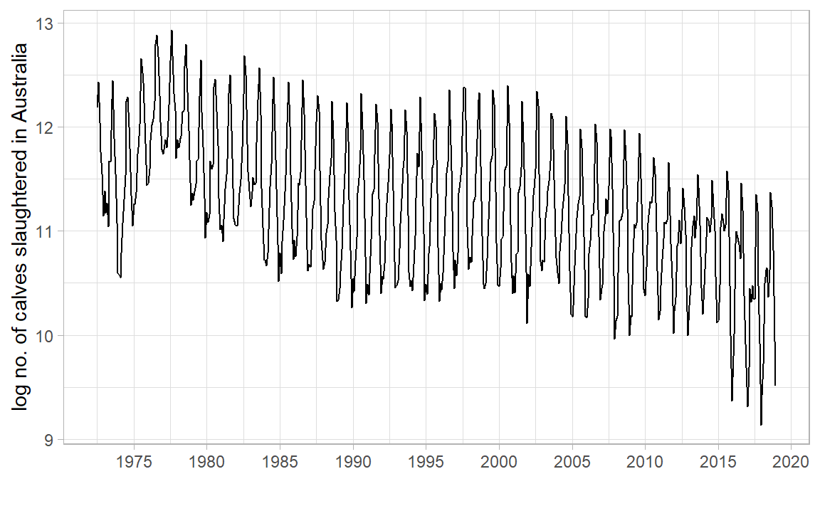
feastsSeamless integration with ggplot2 and friends, use autoplot() from feasts:
|> autoplot (log_count) + labs (x = "" , y = "log no. of calves slaughtered in Australia" ) + scale_x_yearmonth (date_breaks = "5 year" , date_labels = "%Y" ) + theme_light ()
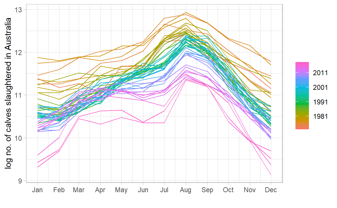
Some more useful plots:
library (feasts)|> gg_season (log_count) + labs (x = "" , y = "log no. of calves slaughtered in Australia" ) + theme_light ()
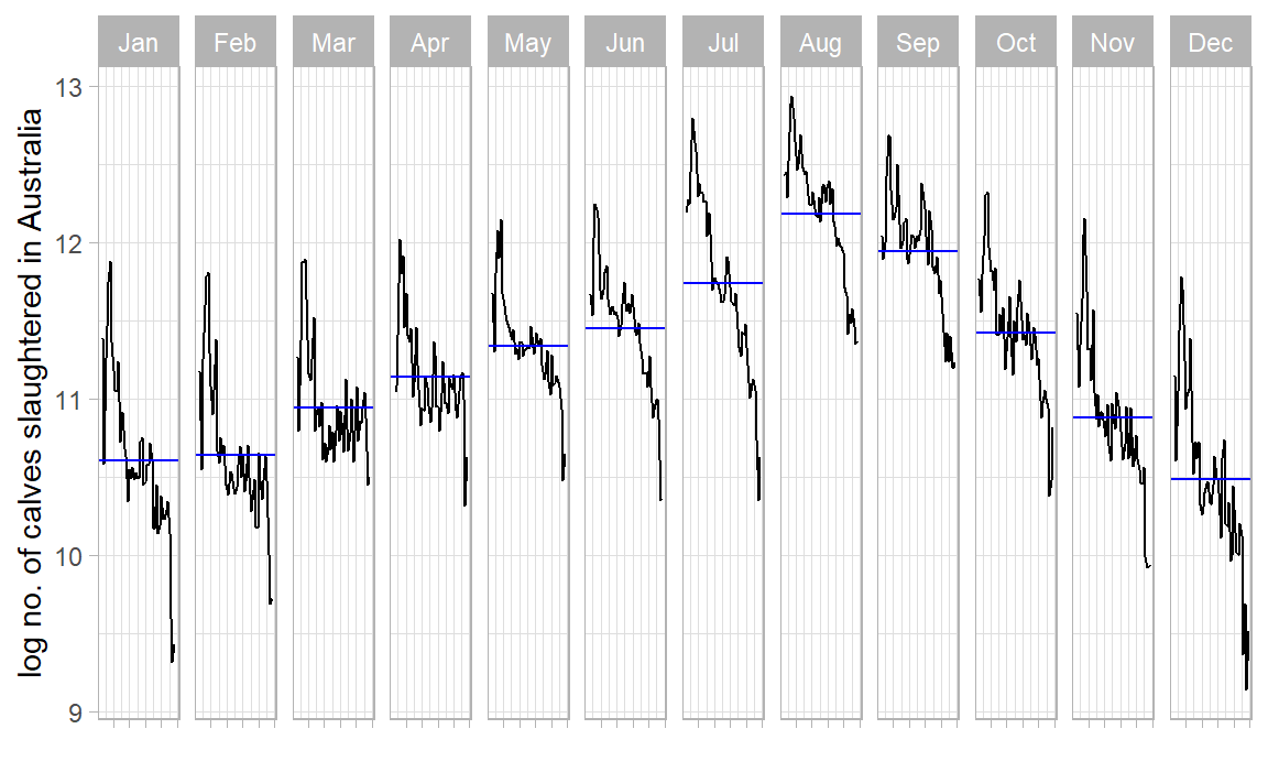
|> gg_subseries (log_count) + labs (x = "" , y = "log no. of calves slaughtered in Australia" ) + scale_x_yearmonth (labels = NULL ) + theme_light ()
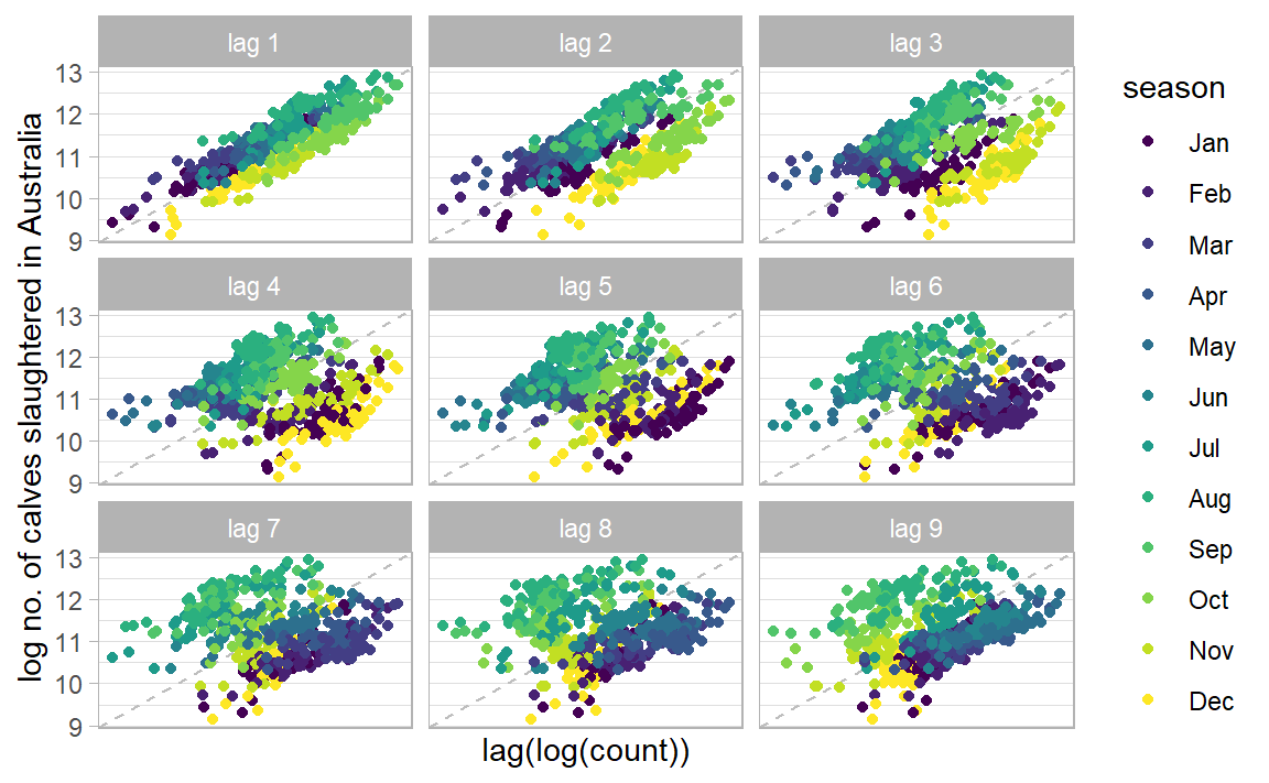
|> gg_lag (log_count, geom = "point" ) + labs (x = "lag(log(count))" , y = "log no. of calves slaughtered in Australia" ) + scale_x_yearmonth (labels = NULL ) + theme_light ()
Some useful features for multiple series:
|> features (log (Count), quantile)
# A tibble: 54 × 7
   Animal                     State            `0%`   `25%`   `50%` `75%` `100%`
   <fct>                      <fct>           <dbl>   <dbl>   <dbl> <dbl>  <dbl>
 1 Bulls, bullocks and steers Australian C… -Inf    -Inf    -Inf     7.60   8.32
 2 Bulls, bullocks and steers New South Wa…   10.8    11.1    11.3  11.4   11.9
 3 Bulls, bullocks and steers Northern Ter… -Inf    -Inf       4.61  7.85   9.74
 4 Bulls, bullocks and steers Queensland      10.5    11.7    11.9  12.1   12.4
 5 Bulls, bullocks and steers South Austra…    8.59    9.59    9.80  9.96  10.4
 6 Bulls, bullocks and steers Tasmania         8.16    8.75    8.95  9.15   9.67
 7 Bulls, bullocks and steers Victoria        10.4    10.8    11.0  11.1   11.8
 8 Bulls, bullocks and steers Western Aust…    8.97    9.62    9.83 10.1   10.7
 9 Calves                     Australian C… -Inf    -Inf    -Inf     4.61   7.17
10 Calves                     New South Wa…    7.60    9.62    9.83 10.0   11.0
# … with 44 more rows
|> group_by (Animal) |> summarise (total_count = sum (Count)) |> features (log (total_count), feat_stl) |> select (Animal, trend_strength, spikiness, linearity)
# A tibble: 7 × 4
  Animal                     trend_strength spikiness linearity
  <fct>                               <dbl>     <dbl>     <dbl>
1 Bulls, bullocks and steers          0.727  8.61e-11    0.0747
2 Calves                              0.945  6.94e-10   -8.02
3 Cattle (excl. calves)               0.818  9.96e-11    0.656
4 Cows and heifers                    0.881  1.56e-10    0.955
5 Lambs                               0.834  1.34e-10    2.35
6 Pigs                                0.930  1.42e-11    2.14
7 Sheep                               0.931  6.26e-10   -4.38
Why did we need log? What would occur without it?
What other transformations are worth considering? Hint: “total monthly sales”
What is the 1st conclusion about no. of calves slaughtered in AUS? What is the 2nd?
Classical Decomposition
Let \(Y_1, \dots, Y_n\) be our TS, then: \[
Y_t = S_t + T_t + e_t
\]
where \(S_t\) is the seasonal component, \(T_t\) is the trend, \(e_t\) is the remainder, all at time \(t\) .
Necessary but not sufficient condition: Make \(e_t\) “white noise”, i.e. \(e_t \stackrel{iid}\sim \mathcal{N}(0, \sigma^2)\)
Decomposition can also be multiplicative:
\[
Y_t = S_t \times T_t \times e_t
\]
but then we’d take \(\log(Y_t)\) .
To make a long story short:
Moving Averages
\(m\) -MA suitable for an odd seasonality period \(m = 2k + 1\) (e.g. a week):
\[
\hat{T}_t = \frac{1}{m}\sum_{j = -k}^{j = k} Y_{t + j}
\]
|> mutate (` 7-MA ` = slider:: slide_dbl (log_count, mean,.before = 3 , .after = 3 , .complete = TRUE )
# A tsibble: 558 x 4 [1M]
      Month  count log_count `7-MA`
      <mth>  <dbl>     <dbl>  <dbl>
 1 1972 Jul 196200      12.2   NA
 2 1972 Aug 250600      12.4   NA
 3 1972 Sep 170100      12.0   NA
 4 1972 Oct 128500      11.8   11.8
 5 1972 Nov 103400      11.5   11.6
 6 1972 Dec  69200      11.1   11.5
 7 1973 Jan  87800      11.4   11.3
 8 1973 Feb  71300      11.2   11.3
 9 1973 Mar  78200      11.3   11.3
10 1973 Apr  62600      11.0   11.5
# … with 548 more rows
Moving Averages of Moving Averages
\(2 \times m\) -MA suitable for an even seasonality period \(m = 2k\) (e.g. quarter):
\[\begin{split}
Q_t = \frac{1}{m}\sum_{j = -(k-1)}^{j = k} Y_{t + j} \\
\hat{T}_t = \frac{1}{2} Q_{t-1} + \frac{1}{2} Q_{t}
\end{split}\]
E.g. for \(m = 4\) (quarter):
\[\begin{split}
\hat{T}_t &= \frac{1}{2} \left[\frac{1}{4}(Y_{t-2} + Y_{t-1} + Y_{t} + Y_{t+1}) + \frac{1}{4}(Y_{t-1} + Y_{t} + Y_{t + 1} + Y_{t+2})\right] \\
&= \frac{1}{8}Y_{t_2} + \frac{1}{4}Y_{t_1} + \frac{1}{4}Y_{t} + \frac{1}{4}Y_{t+1} + \frac{1}{8}Y_{t+2}
\end{split}\]
<- aus_calves |> mutate (` 12-MA ` = slider:: slide_dbl (log_count, mean,.before = 6 , .after = 5 , .complete = TRUE ),` 2x12-MA ` = slider:: slide_dbl (` 12-MA ` , mean,.before = 1 , .after = 0 , .complete = TRUE )
# A tsibble: 558 x 5 [1M]
      Month  count log_count `12-MA` `2x12-MA`
      <mth>  <dbl>     <dbl>   <dbl>     <dbl>
 1 1972 Jul 196200      12.2    NA        NA
 2 1972 Aug 250600      12.4    NA        NA
 3 1972 Sep 170100      12.0    NA        NA
 4 1972 Oct 128500      11.8    NA        NA
 5 1972 Nov 103400      11.5    NA        NA
 6 1972 Dec  69200      11.1    NA        NA
 7 1973 Jan  87800      11.4    11.6      NA
 8 1973 Feb  71300      11.2    11.6      11.6
 9 1973 Mar  78200      11.3    11.6      11.6
10 1973 Apr  62600      11.0    11.6      11.6
# … with 548 more rows
mean (aus_calves$ log_count[1 : 12 ]) + mean (aus_calves$ log_count[2 : 13 ])) / 2 $ ` 2x12-MA ` [8 ]
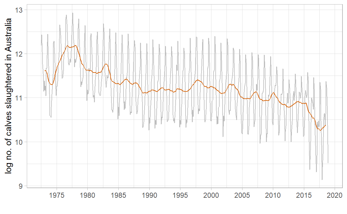
|> autoplot (log_count, colour = "gray" ) + geom_line (aes (y = ` 2x12-MA ` ), colour = "#D55E00" ) + labs (x = "" , y = "log no. of calves slaughtered in Australia" ) + scale_x_yearmonth (date_breaks = "5 year" , date_labels = "%Y" ) + theme_light ()
Back to Classical Decomposition
From Hyndman & Athanasopoulos, 2021 :
If \(m\) is an even number, compute the trend component \(\hat{T}_t\) using a \(2 \times m\) -MA. If \(m\) is an odd number, compute the trend component \(\hat{T}_t\) using a \(m\) -MA.
Calculate the detrended series: \(Y_t - \hat{T}_t\) .
To estimate the seasonal component for each season, simply average the detrended values for that season. These seasonal component values are then adjusted to ensure that they add to zero. The seasonal component is obtained by stringing together these monthly values, and then replicating the sequence for each year of data. This gives \(\hat{S}_t\) .
The remainder component is calculated by subtracting the estimated seasonal and trend-cycle components: \(\hat{e}_t = Y_t - \hat{T}_t - \hat{S}_t\)
In fable:
|> model (classical_decomposition (log_count)) |> components () |> autoplot ()
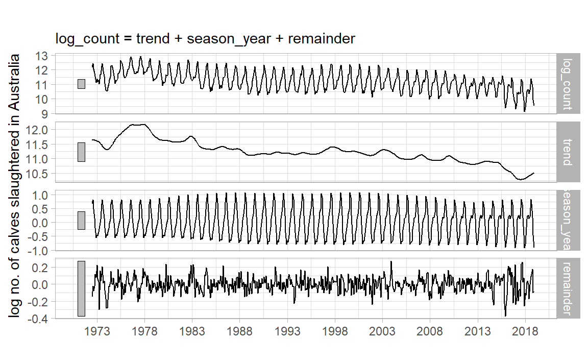
STL Decomposition
STL: Seasonal and Trend decomposition using LOESS, from Clevelnad et al., 1990 .
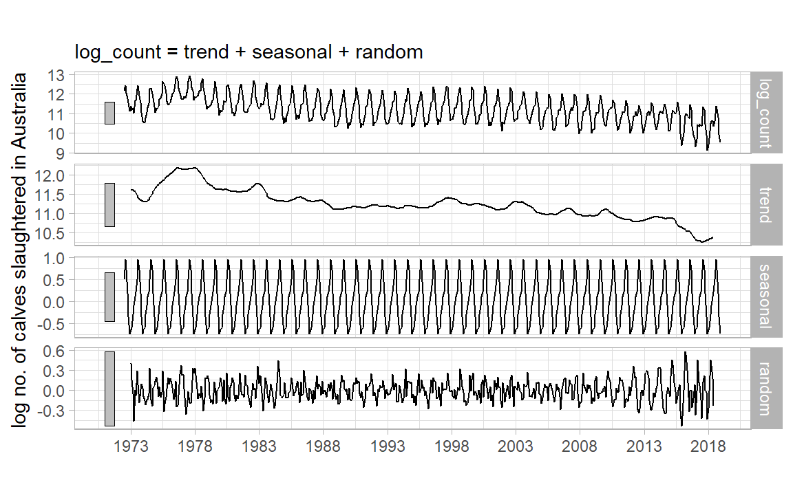
|> model (STL (log_count)) |> components () |> autoplot () + labs (x = "" , y = "log no. of calves slaughtered in Australia" , title = "" ) + scale_x_yearmonth (date_breaks = "5 year" , date_labels = "%Y" ) + theme_light ()
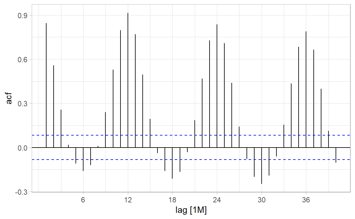
ACF
(Sample) auto-correlation function at lag \(k\) is a huge deal in TSA!
\[
r_k = \frac{\sum_{t = k+1}^{n}(Y_t - \bar{Y})(Y_{t-k} - \bar{Y})}{\sum_{t = 1}^{n} (Y_t - \bar{Y})^2}
\]
|> ACF (log_count, lag_max = 10 )
# A tsibble: 10 x 2 [1M]
        lag      acf
   <cf_lag>    <dbl>
 1       1M  0.844
 2       2M  0.558
 3       3M  0.257
 4       4M  0.0172
 5       5M -0.110
 6       6M -0.160
 7       7M -0.121
 8       8M  0.00978
 9       9M  0.240
10      10M  0.529
|> ACF (log_count, lag_max = 40 ) |> autoplot () + theme_light ()
Where does the CI come from?
Residuals
What do we like to see in residuals?
Uncorrelated
Zero mean
Good to have:
Homoscedasticity
Gaussian
Actually we already wrote this: \(e_t \stackrel{iid}\sim \mathcal{N}(0, \sigma^2)\)
All your knowledge from linear regression comes into play! E.g. what if the mean isn’t zero?
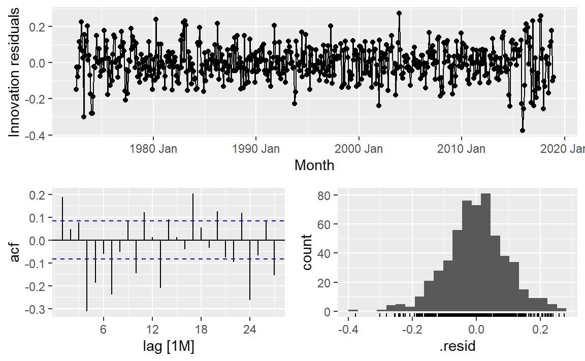
Residuals Diagnostics Viz
Feasts has gg_tsresiduals() for a quick look given a mable:
|> model (STL (log_count)) |> gg_tsresiduals ()
What do you expect to see in each of these?
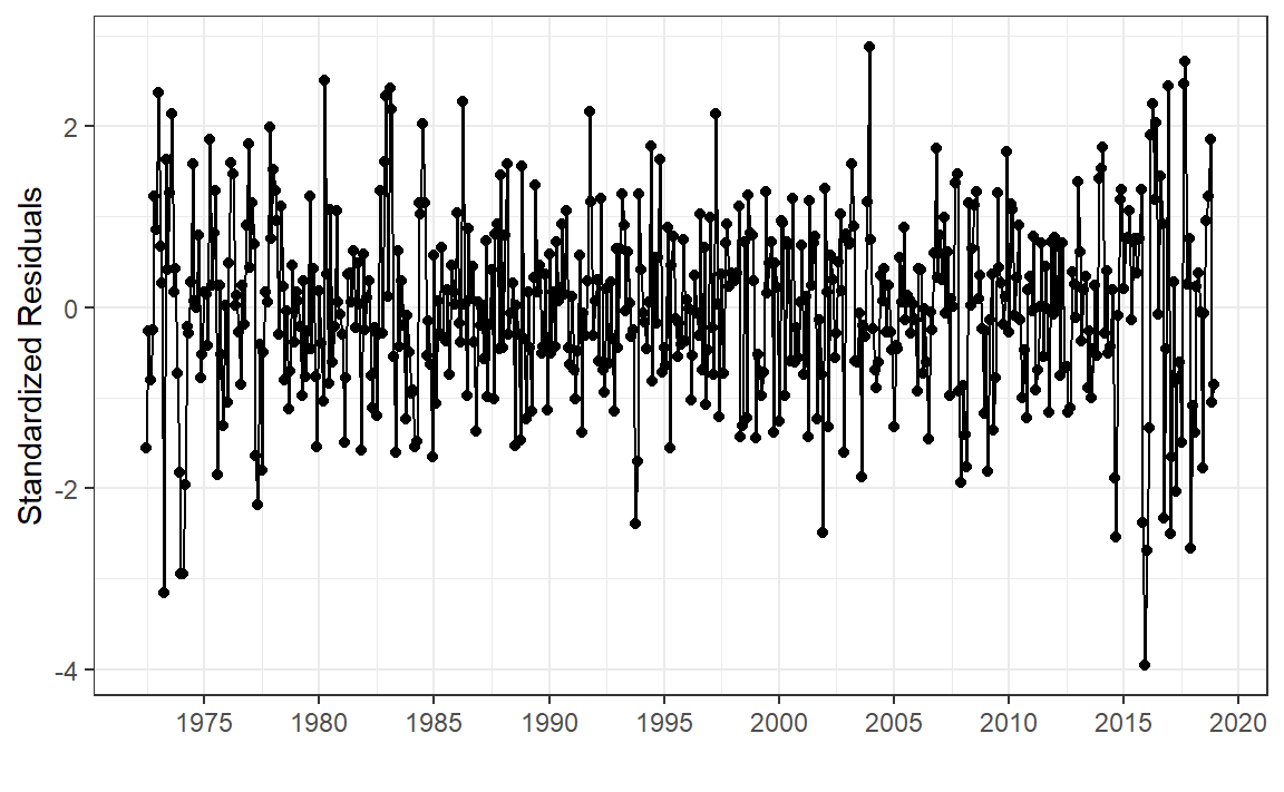
“Stadardized” Residuals Diagnostics Viz
Getting residuals from a fable model (a.k.a mable) with augment():
<- aus_calves |> model (STL (log_count)) |> augment ()
# A tsibble: 558 x 6 [1M]
# Key:       .model [1]
   .model            Month log_count .fitted  .resid  .innov
   <chr>             <mth>     <dbl>   <dbl>   <dbl>   <dbl>
 1 STL(log_count) 1972 Jul      12.2    12.3 -0.149  -0.149
 2 STL(log_count) 1972 Aug      12.4    12.5 -0.0248 -0.0248
 3 STL(log_count) 1972 Sep      12.0    12.1 -0.0772 -0.0772
 4 STL(log_count) 1972 Oct      11.8    11.8 -0.0236 -0.0236
 5 STL(log_count) 1972 Nov      11.5    11.4  0.116   0.116
 6 STL(log_count) 1972 Dec      11.1    11.1  0.0814  0.0814
 7 STL(log_count) 1973 Jan      11.4    11.2  0.226   0.226
 8 STL(log_count) 1973 Feb      11.2    11.1  0.0646  0.0646
 9 STL(log_count) 1973 Mar      11.3    11.2  0.0247  0.0247
10 STL(log_count) 1973 Apr      11.0    11.3 -0.301  -0.301
# … with 548 more rows
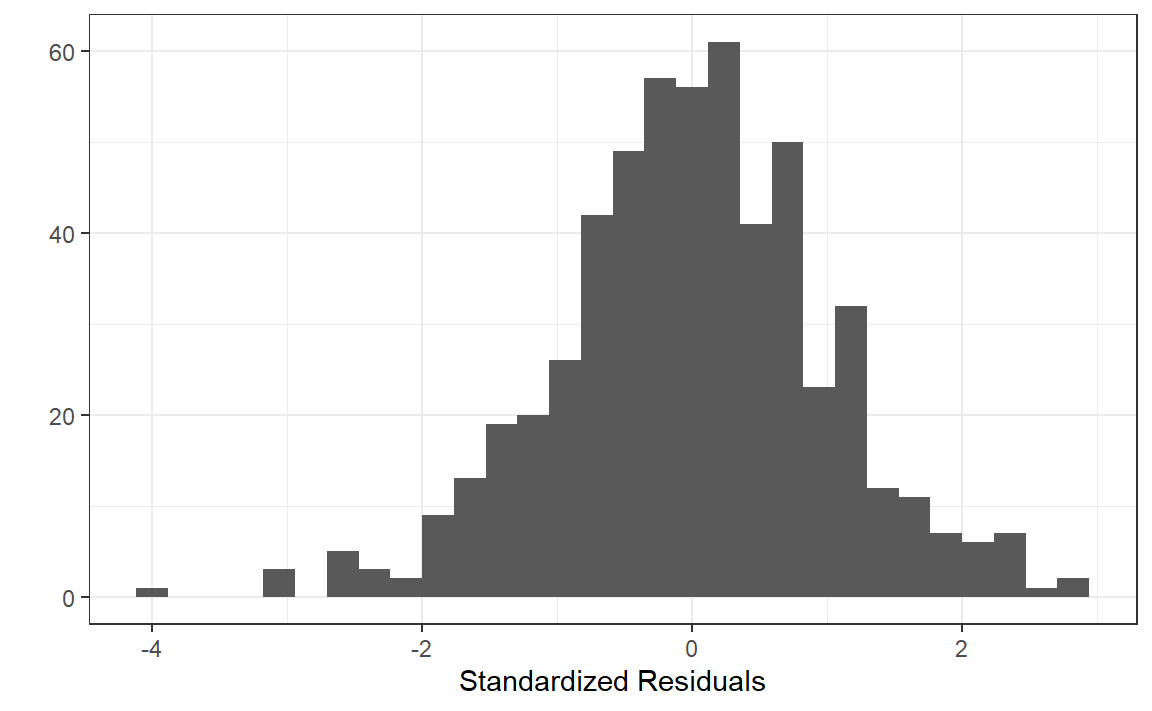
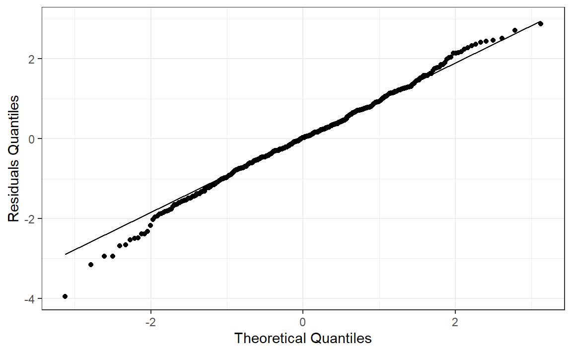
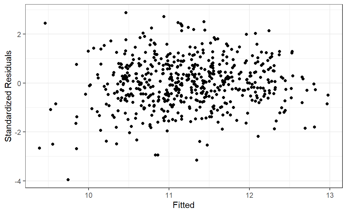
White noise standardized residuals should behave like \(\mathcal{N}(0, 1)\) , so:
<- aus_calves_aug$ .innov<- dim (aus_calves)[1 ]<- sqrt (sum ((resid - mean (resid))** 2 )/ n) # very rough! $ st_resid <- resid / sig
|> ggplot (aes (Month, st_resid)) + geom_point () + geom_line () + labs (x = "" , y = "Standardized Residuals" ) + scale_x_yearmonth (date_breaks = "5 year" , date_labels = "%Y" ) + theme_bw ()
|> ggplot (aes (x = st_resid)) + geom_histogram () + labs (x = "Standardized Residuals" , y = "" ) + theme_bw ()
|> ggplot (aes (sample = st_resid)) + stat_qq () + stat_qq_line () + labs (x = "Theoretical Quantiles" , y = "Residuals Quantiles" ) + theme_bw ()
|> ggplot (aes (.fitted, st_resid)) + geom_point () + labs (x = "Fitted" , y = "Standardized Residuals" ) + theme_bw ()
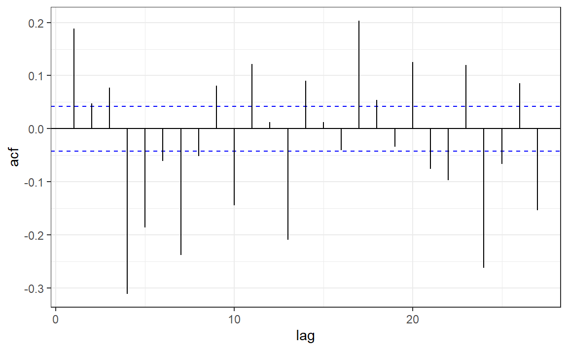
<- acf (aus_calves_aug$ st_resid, plot = FALSE )<- with (acf_obj, tibble (lag = lag[,,1 ], acf = acf[,,1 ])) |> filter (lag > 0 )|> ggplot (aes (lag, acf)) + geom_hline (aes (yintercept = 0 )) + geom_hline (aes (yintercept = - 1 / sqrt (n)), color = "blue" , linetype = 2 ) + geom_hline (aes (yintercept = 1 / sqrt (n)), color = "blue" , linetype = 2 ) + geom_segment (aes (xend = lag, yend = 0 )) + theme_bw ()
Residuals Statistical Tests
Normality - Shapiro-Wilk Test:
shapiro.test (aus_calves_aug$ st_resid)
    Shapiro-Wilk normality test

data:  aus_calves_aug$st_resid
W = 0.99429, p-value = 0.03469
TS independence - Runs Test:
:: runs (aus_calves_aug$ st_resid)
$pvalue
[1] 0.223

$observed.runs
[1] 265

$expected.runs
[1] 279.871

$n1
[1] 273

$n2
[1] 285

$k
[1] 0
ACF - Ljung-Box Test:
\[
Q^* = n(n+2)\sum_{k = 1}^l (n - k)^{-1}r^2_k \sim \chi^2_l
\]
Box.test (aus_calves_aug$ st_resid, lag = 10 , type = "Ljung" )
    Box-Ljung test

data:  aus_calves_aug$st_resid
X-squared = 149.71, df = 10, p-value < 2.2e-16
A bit more tidy with fable:
|> features (.innov, ljung_box, lag = 10 )
# A tibble: 1 × 3
  .model         lb_stat lb_pvalue
  <chr>            <dbl>     <dbl>
1 STL(log_count)    150.         0
Baseline Forecasts
In general, \(\hat{Y}_t(l) = E(Y_{t+l} | Y_1, \dots, Y_t)\) is the minimum MSE forecast, \(l\) time units into the future from time \(t\) .
What if \(Y_t = \mu + e_t\) ?
What if \(Y_t = \mu_t + e_t = \beta_0 + \beta_1\cdot t + e_t\) ?
Mean: \(\hat{Y}_t(l) = \bar{Y}\)
Naive: \(\hat{Y}_t(l) = Y_t\)
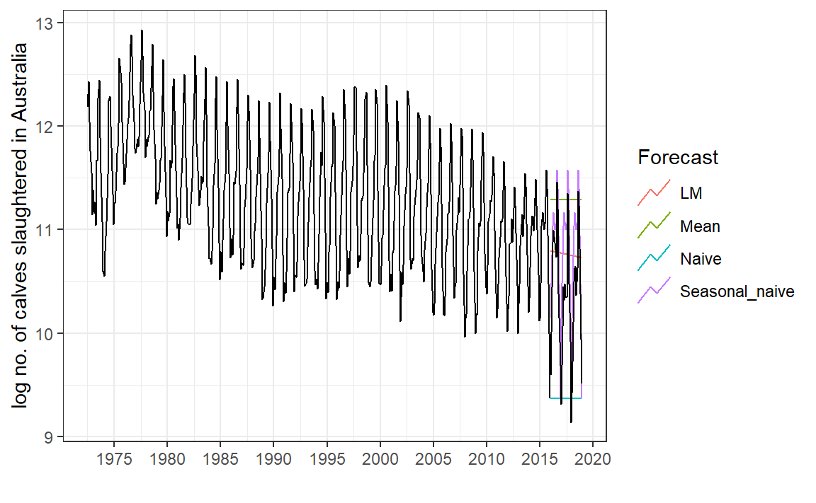
Seasonal Naive: \(\hat{Y}_t(l) = Y_{t + l - m(k-1)}\) , where \(m\) is the seasonality and \(k\) is the integer part of \((l-1)/m\) (i.e. the forecast for all future February values is equal to the last observed February value.)
Linear regression: \(\hat{Y}_t(l) = \hat{\beta}_0 + \hat{\beta}_1(t + l)\)
# Set training data until 2016 <- aus_calves |> filter (year (Month) < 2016 )<- aus_calves |> filter (year (Month) >= 2016 )# Fit the models <- calves_tr |> model (Mean = fable:: MEAN (log_count),Naive = fable:: NAIVE (log_count),Seasonal_naive = fable:: SNAIVE (log_count),LM = fable:: TSLM (log_count ~ trend ())# Generate forecasts for 3 years <- models_fit |> forecast (calves_te)# Can also do forecast(h = 36)
# Plot forecasts against actual values |> autoplot (calves_tr, level = NULL ) + autolayer (filter_index (aus_calves, "2016-01" ~ .),colour = "black" ) + guides (colour = guide_legend (title = "Forecast" )) + labs (x = "" , y = "log no. of calves slaughtered in Australia" ) + scale_x_yearmonth (date_breaks = "5 year" , date_labels = "%Y" ) + theme_bw ()
Evaluating forecast point accuracy
E.g. RMSE, MAE:
|> accuracy (data = calves_te,measures = list ("RMSE" = RMSE, "MAE" = MAE)
# A tibble: 4 × 4
  .model         .type  RMSE   MAE
  <chr>          <chr> <dbl> <dbl>
1 LM             Test  0.718 0.575
2 Mean           Test  1.08  0.904
3 Naive          Test  1.21  1.05
4 Seasonal_naive Test  0.465 0.393