ARIMA

Applications of Data Science - Class 21

Giora Simchoni

`gsimchoni@gmail.com` and add `#dsapps` in subject

Stat. and OR Department, TAU

2023-04-10

Motivation

models_fit <- calves_tr |>
  model(
    Mean = MEAN(log_count),
    Naive = NAIVE(log_count),
    Seasonal_naive = SNAIVE(log_count),
    LM = TSLM(log_count ~ trend()),
    Arima = ARIMA(log_count)
  )

models_fc <- models_fit |> forecast(calves_te)

models_fc |>
  accuracy(
    data = calves_te,
    measures = list("RMSE" = RMSE, "MAE" = MAE)
  )

# A tibble: 5 × 4
  .model         .type  RMSE   MAE
  <chr>          <chr> <dbl> <dbl>
1 Arima          Test  0.290 0.246
2 LM             Test  0.718 0.575
3 Mean           Test  1.08  0.904
4 Naive          Test  1.21  1.05 
5 Seasonal_naive Test  0.465 0.393

Random Processes & Stationarity

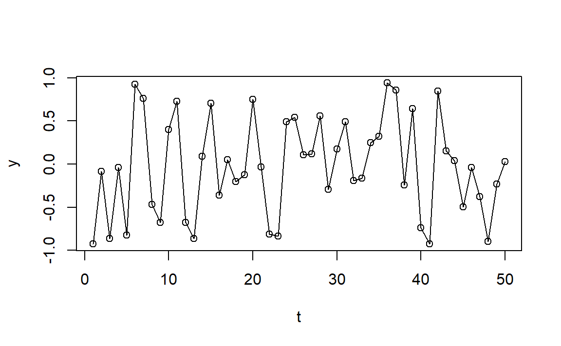
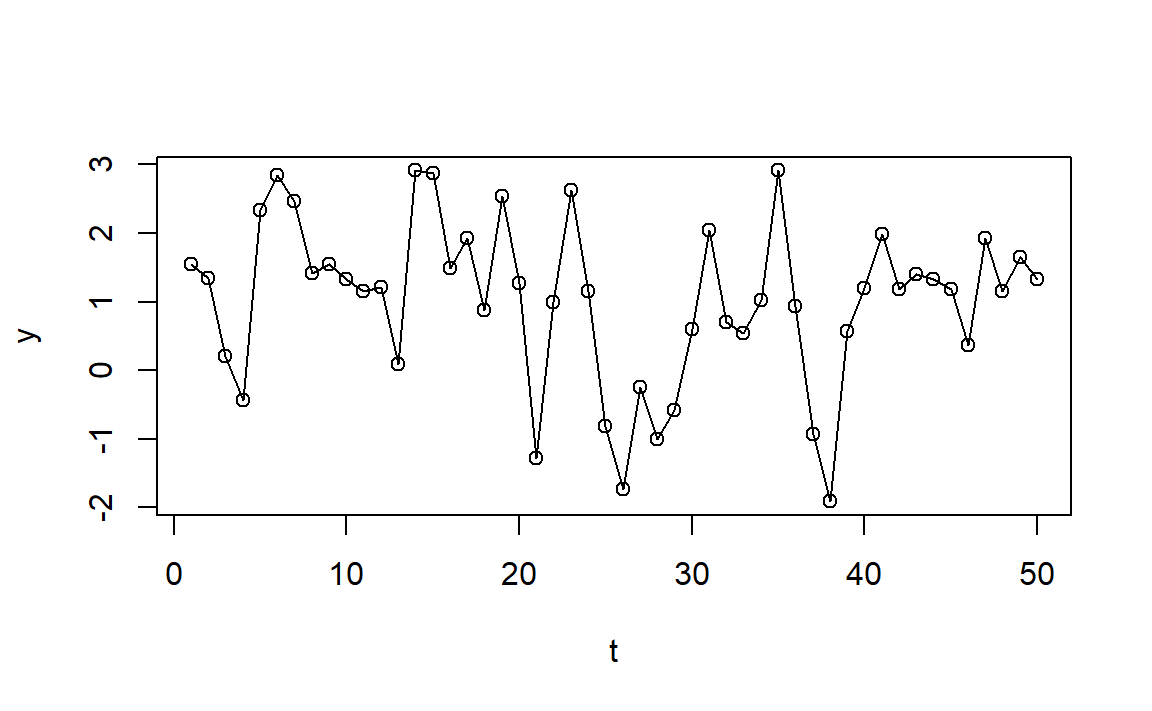
White Noise

\(e_1, e_2, \dots\) are i.i.d RVs with mean 0 and variance \(\sigma^2\), and

\[\begin{aligned} Y_1 &= e_1 \\ Y_2 &= e_2 \\ & \vdots \\ Y_t &= e_t \end{aligned}\]

y <- runif(50, -1, 1)
plot(y, type = "o", xlab = "t")

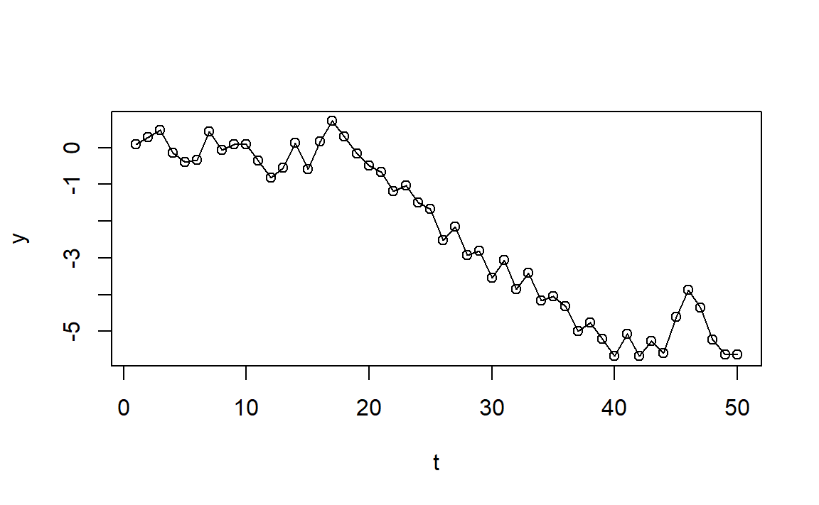
Random Walk

\[\begin{aligned} Y_1 &= e_1 \\ Y_2 &= e_1 + e_2 \\ & \vdots \\ Y_t &= e_1 + \dots + e_t \end{aligned}\]

Or simply: \(Y_t = Y_{t - 1} + e_t\)

y <- cumsum(runif(50, -1, 1))
plot(y, type = "o", xlab = "t")

Simple Moving Average

\[\begin{aligned} Y_2 &= \frac{e_{2} + e_{1}}{2} \\ & \vdots \\ Y_t &= \frac{e_{t} + e_{t-1}}{2} \end{aligned}\]

cy <- cumsum(runif(50, -1, 1))
y <- (cy[2:length(cy)] + cy[1:(length(cy) - 1)]) / 2
plot(y, type = "o", xlab = "t")

Stationarity

“probability laws that govern the behavior of the process do not change over time”
Strong: \(Pr(Y_{t_1} < y_{t_1}, \dots, Y_{t_n} < y_{t_n}) = Pr(Y_{t_1-k} < y_{t_1-k}, \dots, Y_{t_n-k} < y_{t_n-k})\), for all choices of \(t_1, \dots, t_n\) and lag \(k\)
Weak:
1. \(E(Y_{t}) = E(Y_{t + k})\) (mean constant over time)
2. \(Cov(Y_t, Y_{t-k}) = Cov(Y_k, Y_0)\) (covariance depends on lag \(k\) only)
If \(Y_t \sim \mathcal{N}\) strong and weak requirements coincide.

So, which processes are (weakly) stationary?

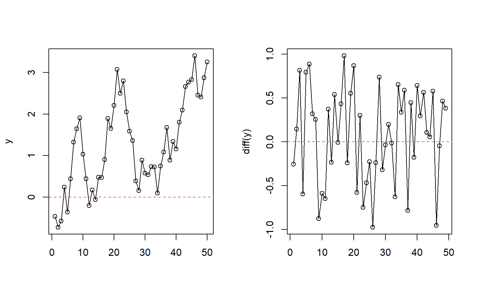
How to “make” Random Walk stationary?

Differencing: \(Y_t - Y_{t - 1} = e_t\)

set.seed(1)
y <- cumsum(runif(50, -1, 1))
par(mfcol = c(1, 2))
plot(y, type = "o", xlab = "")
abline(h = 0, lty = 2, col = 2)
plot(diff(y), type = "o", xlab = "")
abline(h = 0, lty = 2, col = 2)

Autoregessive Processes

AR(p)

An observation \(Y_t\) is a linear combination of past \(p\) most recent observations:

\[ Y_t = \mu + \phi_1 Y_{t-1} + \phi_2 Y_{t-2} + \dots + \phi_p Y_{t-p} + e_t \] where \(e_t\) is an “innovation” term as before, thus \(Cov(e_t, Y_{t-k})=0\) for every \(k > 0\).

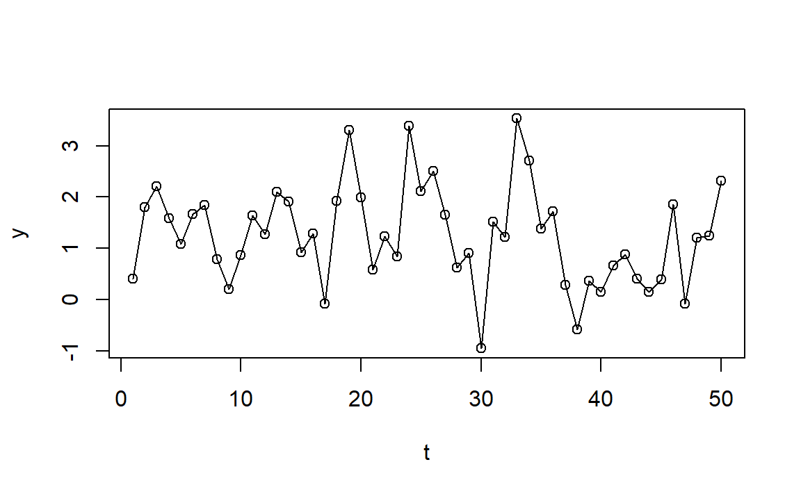
E.g. \(Y_t = 1 + 0.5Y_{t-1} + 0.1Y_{t-2} - 0.1Y_{t-3} + e_t\)

y <- 1 + arima.sim(list(order = c(3,0,0), ar = c(0.5, 0.1, -0.1)), n = 50)
plot(y, type = "o", xlab = "t")

AR(1)

Let the process mean \(\mu\) be subtracted:

\[ Y_t = \phi Y_{t-1} + e_t \]

What if \(\phi = 0\)? What if \(\phi = 1\)?

\(E(Y_t) = \phi E(Y_{t-1}) + E(e_t) = \dots = 0\)

From stationarity:

\(Var(Y_t) = \phi^2Var(Y_t) + \sigma^2 \rightarrow Var(Y_t) = \frac{\sigma^2}{1-\phi^2}\)

So \(|\phi| < 1\).

AR(1)

\[\begin{aligned} Cov(Y_t, Y_{t-k}) &= E(Y_t Y_{t-k}) - E(Y_t)E(Y_{t-k}) \\ &= \phi E(Y_{t-1} Y_{t-k}) - E(e_t Y_{t-k}) \\ & \vdots \\ &= \phi^k Var(Y_t) = \phi^k \frac{\sigma^2}{1-\phi^2} \end{aligned}\]

\[ \rho_k = Corr(Y_t, Y_{t-k}) = \frac{Cov(Y_t, Y_{t-k})}{\sqrt{Var(Y_t)}\sqrt{Var(Y_{t-k})}} = \phi^k \]

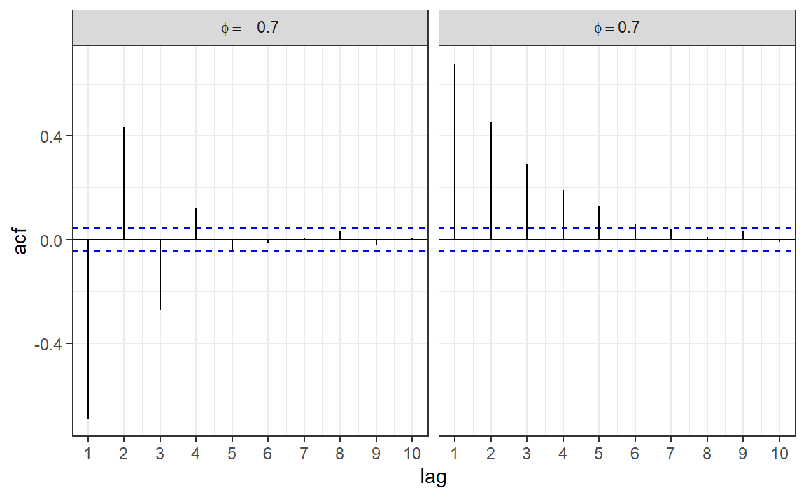
How would the ACF look like?

Is AR(1) (weakly) stationary?

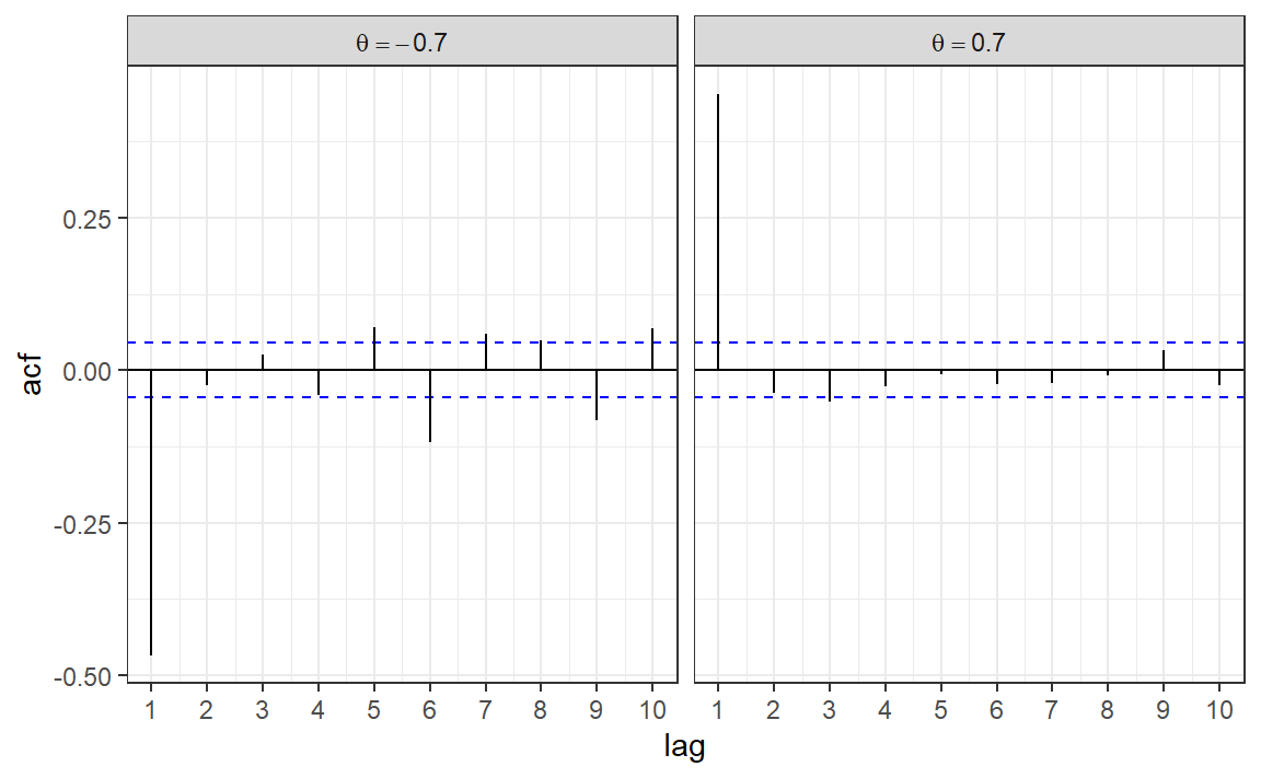
AR(1) - ACF

Code

set.seed(1)
n <- 500
y_pos <- arima.sim(list(order = c(1,0,0), ar = 0.7), n = n)
y_neg <- arima.sim(list(order = c(1,0,0), ar = -0.7), n = n)
acf_df_pos <- make_acf_df(y_pos)
acf_df_neg <- make_acf_df(y_neg)
acf_df_pos$phi <- "phi == 0.7"
acf_df_neg$phi <- "phi == -0.7"
acf_df <- bind_rows(acf_df_pos, acf_df_neg)

acf_df |>
  ggplot(aes(lag, acf)) +
  geom_hline(aes(yintercept = 0)) +
  geom_hline(aes(yintercept = -1/sqrt(n)), color = "blue", linetype = 2) +
  geom_hline(aes(yintercept = 1/sqrt(n)), color = "blue", linetype = 2) +
  geom_segment(aes(xend = lag, yend = 0)) +
  facet_grid(. ~ phi, labeller = labeller(phi = label_parsed)) +
  scale_x_continuous(breaks = 1:10) +
  theme_bw()

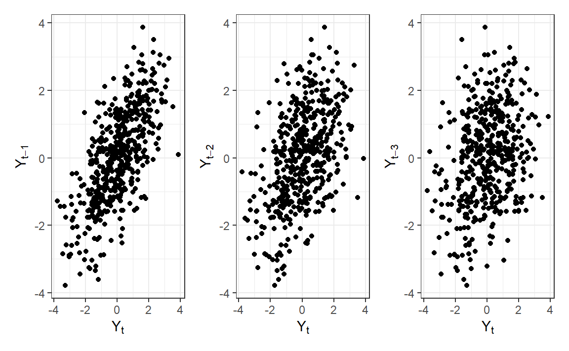
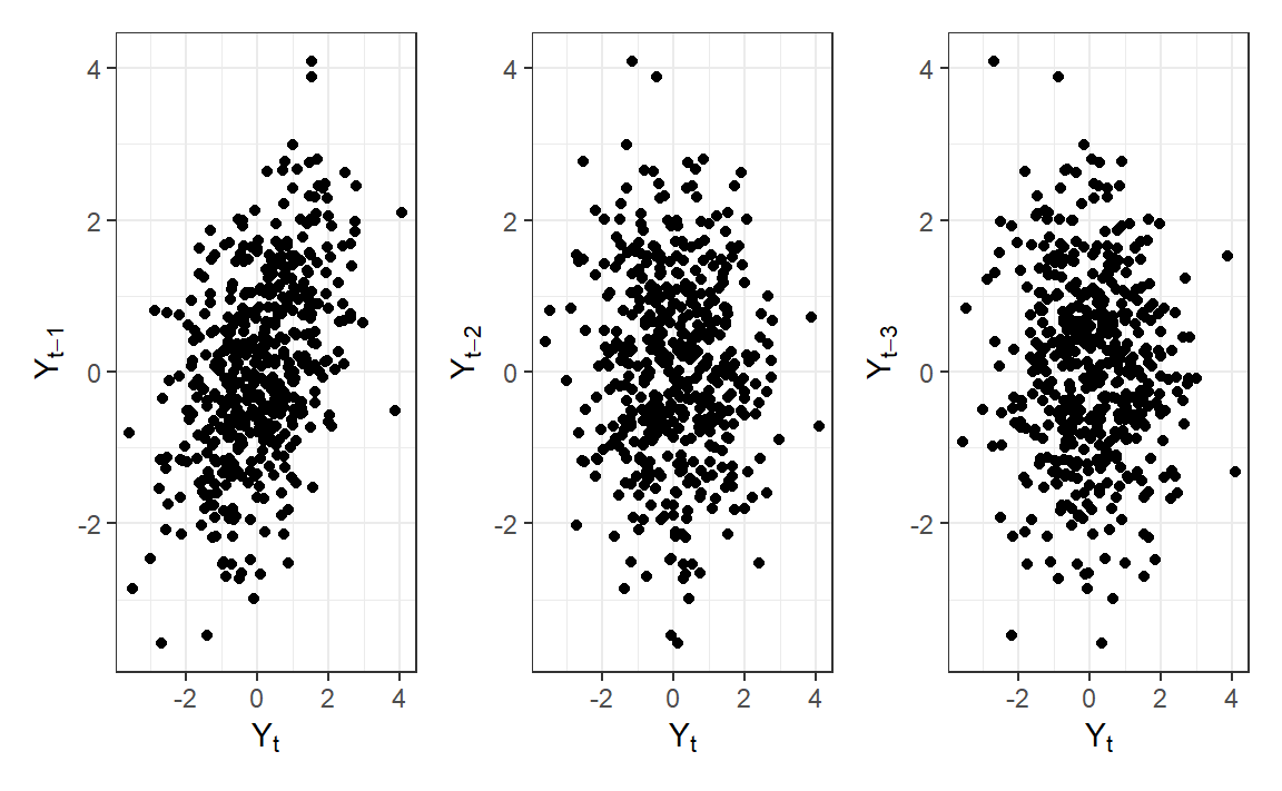
AR(1) - Lag Scatterplots

Code

library(patchwork)

y_lag_df <- tibble(
  y = y_pos,
  y_lag1 = TSA::zlag(y_pos, 1),
  y_lag2 = TSA::zlag(y_pos, 2),
  y_lag3 = TSA::zlag(y_pos, 3)
)
p1 <- ggplot(y_lag_df, aes(y, y_lag1)) +
  geom_point() +
  labs(x = expression("Y"[t]), y = expression("Y"[t-1])) +
  theme_bw()
p2 <- ggplot(y_lag_df, aes(y, y_lag2)) +
  geom_point() +
  labs(x = expression("Y"[t]), y = expression("Y"[t-2])) +
  theme_bw()
p3 <- ggplot(y_lag_df, aes(y, y_lag3)) +
  geom_point() +
  labs(x = expression("Y"[t]), y = expression("Y"[t-3])) +
  theme_bw()

p1|p2|p3

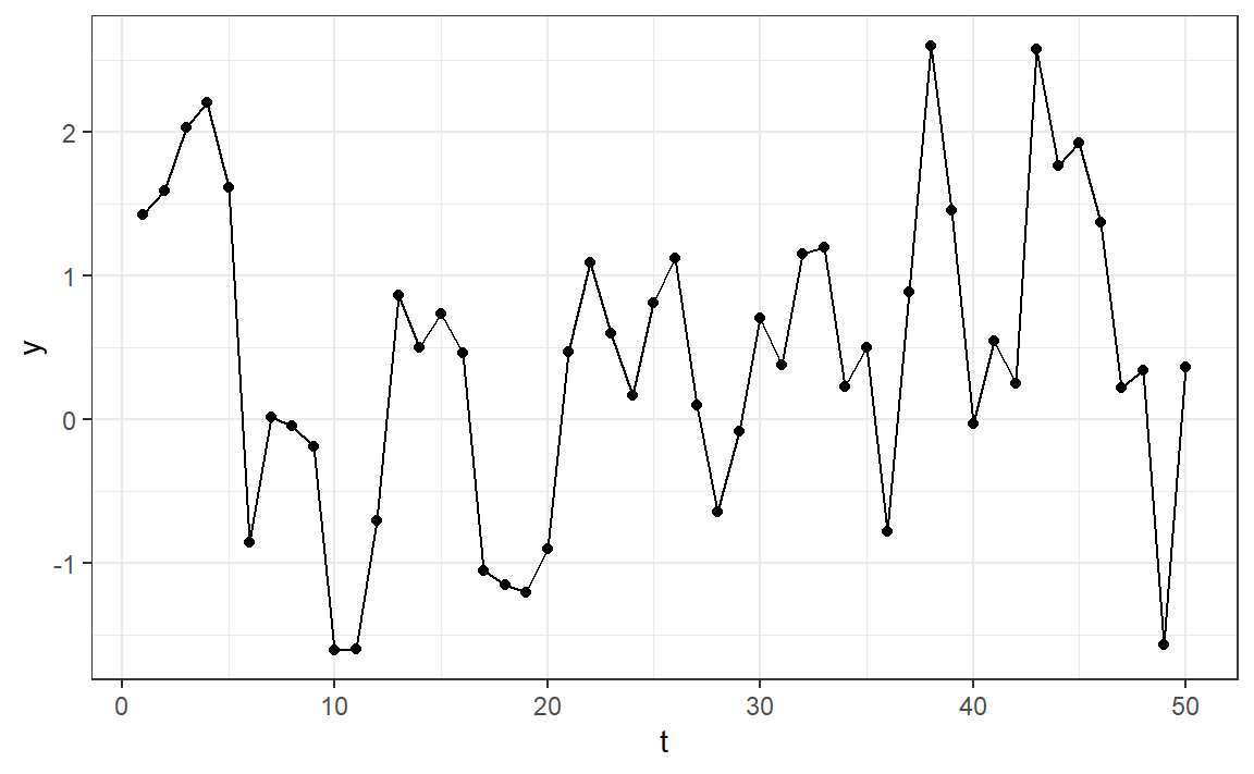
So will you recognize an AR(1) TS when you see it?

tibble(t = 1:50, y = y_pos[1:50]) |>
  ggplot(aes(t, y)) +
  geom_line() +
  geom_point() +
  theme_bw()

AR(2)

\[ Y_t = \phi_1 Y_{t-1} + \phi_2 Y_{t-2} + e_t \]

\(E(Y_t) = \phi_1 E(Y_{t-1}) + \phi_2 E(Y_{t-2}) + E(e_t) = \dots = 0\)

From stationarity \(\gamma_k = Cov(Y_{t}, Y_{t-k})\) for any \(t, k\), so:

\[\begin{aligned} \gamma_0 = Var(Y_t) &= \phi_1^2Var(Y_{t-1}) + \phi_2^2Var(Y_{t-2}) + 2\phi_1\phi_2Cov(Y_{t-1}, Y_{t-2}) + \sigma^2 \\ & = (\phi_1^2 + \phi_2^2)\gamma_0 + 2\phi_1\phi_2\gamma_1 + \sigma^2 \end{aligned}\]

On the other hand:

\[\begin{aligned} \gamma_1 = Cov(Y_{t}, Y_{t-1}) = E(Y_{t}\cdot Y_{t-1}) &= E([\phi_1 Y_{t-1} + \phi_2 Y_{t-2} + e_t] \cdot Y_{t-1}) \\ &= \phi_1E(Y^2_{t-1}) + \phi_2Cov(Y_{t-1}, Y_{t-2}) = \phi_1\gamma_0 + \phi_2\gamma_1 \end{aligned}\]

Giving… \(\gamma_0 = Var(Y_t) = \left(\frac{1-\phi_2}{1+\phi_2}\right)\frac{\sigma^2}{(1-\phi_2)^2-\phi_1^2}\)

AR(2)

In the same way we can show for any \(k\):

\[ \gamma_k = Cov(Y_t, Y_{t-k}) = \phi_1\gamma_{k-1} + \phi_2\gamma_{k-2} \]

\[ \rho_k = Corr(Y_t, Y_{t-k}) = \frac{Cov(Y_t, Y_{t-k})}{\sqrt{Var(Y_t)}\sqrt{Var(Y_{t-k})}} = \phi_1\rho_{k-1} + \phi_2\rho_{k-2} \]

The Yule-Walker equations! Though there is a closed form.

Counting on \(\rho_0 = 1\) and \(\rho_{-1} = \rho_1\), we get:

\[ \rho_1 = \frac{\phi_1}{1-\phi_2}; \quad \rho_2 = \frac{\phi_2(1-\phi_2) + \phi_1^2}{1-\phi_2}; \]

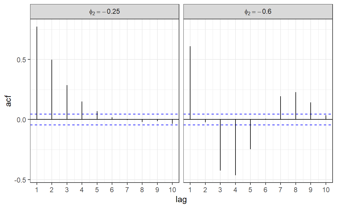
AR(2) - ACF

Here \(\phi_1 = 1\) in both TS:

Code

set.seed(1)
n <- 500
y_pos <- arima.sim(list(order = c(2,0,0), ar = c(1.0, -0.25)), n = n)
y_neg <- arima.sim(list(order = c(2,0,0), ar = c(1.0, -0.6)), n = n)
acf_df_pos <- make_acf_df(y_pos)
acf_df_neg <- make_acf_df(y_neg)
acf_df_pos$phi <- "phi[2] == -0.25"
acf_df_neg$phi <- "phi[2] == -0.6"
acf_df <- bind_rows(acf_df_pos, acf_df_neg)

acf_df |>
  ggplot(aes(lag, acf)) +
  geom_hline(aes(yintercept = 0)) +
  geom_hline(aes(yintercept = -1/sqrt(n)), color = "blue", linetype = 2) +
  geom_hline(aes(yintercept = 1/sqrt(n)), color = "blue", linetype = 2) +
  geom_segment(aes(xend = lag, yend = 0)) +
  facet_grid(. ~ phi, labeller = labeller(phi = label_parsed)) +
  scale_x_continuous(breaks = 1:10) +
  theme_bw()

Stationarity Conditions

In AR(1) we only needed \(|\phi| < 1\).

In AR(2), for example, from \(\rho_1 = \frac{\phi_1}{1-\phi_2}\) it is clear that if \(\phi_2 < 1\): \(\phi_1 + \phi_2 < 1\) and \(\phi_2 - \phi_1 < 1\)

In general it can be shown that for AR(p) to be stationary the characteristic equation \(1-\phi_1x-\phi_2x^2- \dots -\phi_px^p = 0\) needs \(p\) roots above 1 in absolute value.

For AR(1): \(1-\phi x = 0 \rightarrow |1/\phi| > 1 \rightarrow |\phi| < 1\)

For AR(2): \(1-\phi_1x-\phi_2x^2 = 0 \rightarrow \left|\frac{\phi_1 \pm \sqrt{\phi_1^2 + 4\phi_2}}{-2\phi_2}\right| > 1 \rightarrow \phi_1 + \phi_2 < 1, \phi_2 - \phi_1 < 1, |\phi_2| < 1\)

Unit Root Tests

In general, the roots must lie outside the unit circle in the complex plane, hence we have unit-roots tests, to test for stationarity:

# Augmented Dicky-Fuller (ADF) Test, H0: non-stationary
tseries::adf.test(y_pos, k = 0)


    Augmented Dickey-Fuller Test

data:  y_pos
Dickey-Fuller = -7.8867, Lag order = 0, p-value = 0.01
alternative hypothesis: stationary

# KPSS Test, H0: stationary
unitroot_kpss(y_pos)

  kpss_stat kpss_pvalue 
  0.1039691   0.1000000

See also unitroot_ndiffs() in fable for determining how many diffs are needed for stationarity.

Moving Average Processes

MA(q)

An observation \(Y_t\) is a linear combination of past \(q\) most recent errors:

\[ Y_t = \mu + e_t + \theta_1 e_{t-1} + \theta_2 e_{t-2} + \dots + \theta_q e_{t-q} \] where \(e_t\) is an “innovation” term as before.

E.g. \(Y_t = 1 + e_t + 0.5e_{t-1} + 0.1e_{t-2} - 0.1e_{t-3}\)

y <- 1 + arima.sim(list(order = c(0,0,3), ma = c(0.5, 0.1, -0.1)), n = 50)
plot(y, type = "o", xlab = "t")

MA(1)

Let the process mean \(\mu\) be subtracted:

\[ Y_t = e_t + \theta e_{t-1} \]

\(E(Y_t) = E(e_t) + \theta E(e_{t-1}) = 0\)

\(\gamma_0 = Var(Y_t) = Var(e_t) + \theta^2Var(e_{t-1}) = (1+\theta^2)\sigma^2\)

\(\gamma_1 = Cov(Y_t, Y_{t-1}) = Cov(e_t + \theta e_{t-1}, e_{t-1} + \theta e_{t-2}) = \theta\sigma^2\)

\(\rho_1 = \frac{\gamma_1}{\gamma_0} = \frac{\theta}{1+\theta^2}\)

What would be \(\gamma_k, \rho_k\) for \(k > 1\)? How would the ACF look like?

Is MA(1) (weakly) stationary?

MA(1) - ACF

Code

set.seed(1)
n <- 500
y_pos <- arima.sim(list(order = c(0,0,1), ma = 0.7), n = n)
y_neg <- arima.sim(list(order = c(0,0,1), ma = -0.7), n = n)
acf_df_pos <- make_acf_df(y_pos)
acf_df_neg <- make_acf_df(y_neg)
acf_df_pos$phi <- "theta == 0.7"
acf_df_neg$phi <- "theta == -0.7"
acf_df <- bind_rows(acf_df_pos, acf_df_neg)

acf_df |>
  ggplot(aes(lag, acf)) +
  geom_hline(aes(yintercept = 0)) +
  geom_hline(aes(yintercept = -1/sqrt(n)), color = "blue", linetype = 2) +
  geom_hline(aes(yintercept = 1/sqrt(n)), color = "blue", linetype = 2) +
  geom_segment(aes(xend = lag, yend = 0)) +
  facet_grid(. ~ phi, labeller = labeller(phi = label_parsed)) +
  scale_x_continuous(breaks = 1:10) +
  theme_bw()

MA(1) - Lag Scatterplots

Code

library(patchwork)

y_lag_df <- tibble(
  y = y_pos,
  y_lag1 = TSA::zlag(y_pos, 1),
  y_lag2 = TSA::zlag(y_pos, 2),
  y_lag3 = TSA::zlag(y_pos, 3)
)
p1 <- ggplot(y_lag_df, aes(y, y_lag1)) +
  geom_point() +
  labs(x = expression("Y"[t]), y = expression("Y"[t-1])) +
  theme_bw()
p2 <- ggplot(y_lag_df, aes(y, y_lag2)) +
  geom_point() +
  labs(x = expression("Y"[t]), y = expression("Y"[t-2])) +
  theme_bw()
p3 <- ggplot(y_lag_df, aes(y, y_lag3)) +
  geom_point() +
  labs(x = expression("Y"[t]), y = expression("Y"[t-3])) +
  theme_bw()

p1|p2|p3

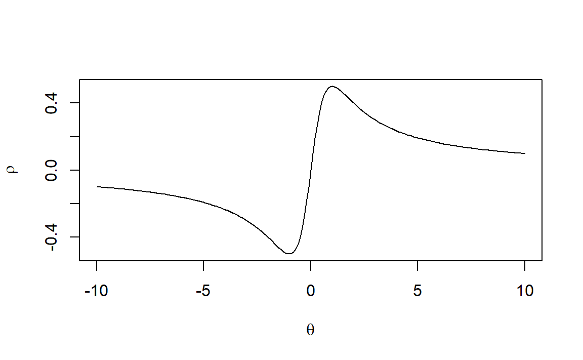
MA(1) - Inveritibility

Can \(\theta\) be any number? Can \(\rho\) be any correlation?

theta <- seq(-10, 10, 0.1)
rho <- theta / (1 + theta^2)
plot(theta, rho, type = "l", xlab = expression(theta), ylab = expression(rho))

\(\rho\) is in \((-\frac{1}{2}, \frac{1}{2})\)

\(|\theta| < 1\), otherwise the model is not identifiable.

MA(1) - Inveritibility

Actually, every MA(q) process can be written as AR(\(\infty\))!

\[\begin{aligned} Y_t = e_t + \theta e_{t-1} &= e_t + \theta (Y_{t-1} - \theta e_{t-2}) \\ &= e_t + \theta Y_{t-1} - \theta^2 (Y_{t-2} - \theta e_{t-3}) \\ &\vdots \\ &= e_t + \theta Y_{t-1} - \theta^2 Y_{t-2} - \theta^3 Y_{t-3} - \dots \end{aligned}\]

Thus, having \(|\theta| < 1\) is called invertibility condition and is very similar to stationarity conditions.

And, every AR(p) model can be written as MA(\(\infty\)).

In general it can be shown that for MA(q) to be invertible the characteristic equation \(1-\theta_1x-\theta_2x^2- \dots -\theta_qx^q = 0\) needs \(q\) roots above 1 in absolute value.

ARIMA

ARMA(p, q)

A mixed autoregressive moving average process (ARMA):

\[ Y_t = \mu + \phi_1 Y_{t-1} + \dots + \phi_p Y_{t-p} + \theta_1 e_{t-1} + \theta_2 e_{t-2} + \dots + \theta_q e_{t-q} + e_t \]

ARMA(1, 1)

Let the process mean \(\mu\) be subtracted:

\[ Y_t = \phi Y_{t-1} + e_t + \theta e_{t-1} \]

\(E(Y_t) = 0\)

\(\gamma_0 = Var(Y_t) = \phi^2 \gamma_0 + (1+\theta^2)\sigma^2 + 2\phi\theta Cov(Y_{t-1}, e_{t-1}) \rightarrow \gamma_0 = \frac{(1+2\phi\theta + \theta^2)}{1-\phi^2}\sigma^2\)

\(\gamma_1 = \phi\gamma_0+\theta\sigma^2\)

\(\gamma_k = \phi\gamma_{k-1} \quad k \ge 2\)

\(\rho_k = \frac{(1+\theta\phi)(\phi+\theta)}{1+2\theta\phi + \theta^2}\phi^{k-1}\)

ARIMA(p, d, q)

\(Y_t\) follows an integrated autoregressive moving average (non-seasonal) ARIMA(p, d, q) model if \(W_t = \nabla^d Y_t\) is a stationary ARMA(p, q) process.

\[ W_t = \mu + \phi_1 W_{t-1} + \dots + \phi_p W_{t-p} + \theta_1 e_{t-1} + \theta_2 e_{t-2} + \dots + \theta_q e_{t-q} + e_t \]

\(p\): order of the autoregressive part
\(d\): degree of first differencing involved
\(q\): order of the moving average part

Usually \(d\) is in \(\{0,1,2\}\).

What are ARIMA(0,0,0), ARIMA(0,1,0), ARIMA(p,0,0), ARIMA(0,0,q)?

Estimation

Least Squares: AR(1)

Putting back the \(\mu\) to estimate it:

\[ Y_t - \mu = \phi (Y_{t-1} - \mu) + e_t \]

This is simple linear regression of \(Y_t\) versus \(Y_{t-1}\)

\[ SS(\mu, \phi) = \sum_{t=2}^n[(Y_t - \mu) - \phi (Y_{t-1} - \mu)]^2 \] Differentiating, setting this equal to zero, we get:

\(\hat{\mu}_{LS} \approx \bar{Y}\)

\(\hat{\phi}_{LS} \approx r_1\)

Least Squares: MA(1)

\[ Y_t - \mu = e_t + \theta e_{t-1} \]

This isn’t simple linear regression, as \(e_t\) aren’t observed!

Option 1: invert MA(1) to AR(\(\infty\)) and use numerical analysis: \[ SS(\mu, \theta) = \sum_{t=2}^n[(Y_t - \mu) - (\theta Y_{t-1} - \theta^2 Y_{t-2} - \theta^3 Y_{t-3} - \dots)]^2 \] Option 2: simple grid search on \(\theta \in (-1, 1)\) to get the minimum \(SS(\theta) = \sum e_t^2\), where:

\[\begin{aligned} e_1 &= Y_1 \\ e_2 &= Y_2 - \theta e_1 \\ &\vdots \\ e_n &= Y_n - \theta e_{n-1} \end{aligned}\]

MLE: AR(1)

Assume \(e_t \sim \mathcal{N}(0, \sigma^2)\) i.i.d.

Is this true: \(L(\mu, \phi, \sigma^2| y) = \prod_{t=1}^n f(y_t; \mu, \phi, \sigma^2) = \prod_{t=1}^n \mathcal{N}(\mu, \frac{\sigma^2}{1-\phi^2})\)

The \(Y_t\)s are dependent!

E.g. \(\rho_1 = \phi\).

They are, however conditionally independent:

\[\begin{aligned} Y_2 &= \mu + \phi(Y_1 - \mu) + e_2 \\ Y_3 &= \mu + \phi(Y_2 - \mu) + e_3 \\ &\vdots \\ Y_n &= \mu + \phi(Y_{n-1} - \mu) + e_n \end{aligned}\]

So: \(f(y_1, y_2, \dots, y_n) = f(y_1)f(y_2|y_1)\cdot \dots \cdot f(y_n|y_{n-1})\)

MLE: AR(1)

Now, \(Y_1 \sim \mathcal{N}(\mu, \frac{\sigma^2}{1-\phi^2})\)

From basic Gaussian probability, if \(X \sim \mathcal{N}(\mu_x, \sigma^2_x), Y \sim \mathcal{N}(\mu_y, \sigma^2_y)\), then

\(Y|X \sim \mathcal{N}(\mu_y + \rho\frac{\sigma_y}{\sigma_x}(x - \mu_x), \sigma^2_y(1-\rho^2))\)

So: \(Y_t | Y_{t-1} \sim \mathcal{N}(\mu + \phi(y_{t-1} - \mu), \sigma^2)\)

After some algebra:

\[ l(\mu, \phi, \sigma^2| y) = -\frac{n}{2}\log(2\pi) -\frac{n}{2}\log(\sigma^2) +\frac{1}{2}(1-\phi^2) \\ -\frac{1}{2\sigma^2}\sum_{t=2}^n [y_t - \mu - \phi(y_{t-1} - \mu)]^2 - (1-\phi^2)(y_1 - \mu)^2 \]

But that sum of squares is exactly \(SS(\mu, \phi)\) for LS + a single term, thus:

\(\hat{\mu}_{MLE} \approx \hat{\mu}_{LS} \quad \hat{\phi}_{MLE} \approx \hat{\phi}_{LS} \quad \hat{\sigma}^2_{MLE} = \frac{SS(\hat{\mu}, \hat{\phi})}{n}\)

y <- arima.sim(list(order = c(1,0,0), ar = 0.5), n = 50)

tsibble(y, t = days(1:50), index = t) |>
  model(ar1 = ARIMA(y ~ pdq(1,0,0))) |> report()

Series: y 
Model: ARIMA(1,0,0) 

Coefficients:
         ar1
      0.4971
s.e.  0.1241

sigma^2 estimated as 1.068:  log likelihood=-72.22
AIC=148.45   AICc=148.7   BIC=152.27

ar(y, order.max = 1, aic = FALSE, method = "mle")


Call:
ar(x = y, aic = FALSE, order.max = 1, method = "mle")

Coefficients:
     1  
0.4893  

Order selected 1  sigma^2 estimated as  1.043

ar(y, order.max = 1, aic = FALSE, method = "ols", intercept=FALSE)


Call:
ar(x = y, aic = FALSE, order.max = 1, method = "ols", intercept = FALSE)

Coefficients:
     1  
0.4692  

Order selected 1  sigma^2 estimated as  1.001

Model Selection

The Old Art of Model Selection

In all TS books there would appear a table similar to this:

	AR(p)	MA(q)	ARMA(p, q)
ACF	Tails off	Cuts off after lag q	Tails off
PACF	Cuts off after lag p	Tails off	Tails off

The advantage is avoiding overfitting.

The disadvantages: time consuming, not accurate, hard to generalize to seasonal ARIMA

AIC, AICc

\[ AIC = -2l + 2(p + q + k + 1) \] where \(l\) is the log-likelihood and \(k = 1\) if the mean \(\mu\) was estimated, otherwise \(k = 0\).

\[ AIC_c = AIC + \frac{2(p+q+k+1)(p+q++k+2)}{n - p - q - k - 2} \]

Do not use AIC to decide on difference order \(d\).

ARIMA in `fable`

See Hyndman & Athanasopoulos.

ARIMA in `fable`

aus_calves |>
  model(
    Arima = ARIMA(log_count)
  ) |>
  report()

Series: log_count 
Model: ARIMA(1,0,1)(2,1,2)[12] w/ drift 

Coefficients:
         ar1      ma1    sar1     sar2     sma1   sma2  constant
      0.8784  -0.2558  0.7841  -0.4800  -1.2514  0.531   -0.0022
s.e.  0.0269   0.0560  0.0955   0.0675   0.1007  0.076    0.0012

sigma^2 estimated as 0.01716:  log likelihood=333.47
AIC=-650.95   AICc=-650.68   BIC=-616.53

You always need to perform Residuals Diagnostics.

Practical Modeling

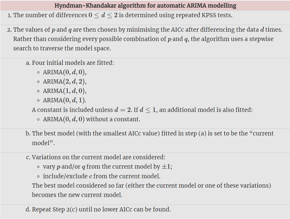
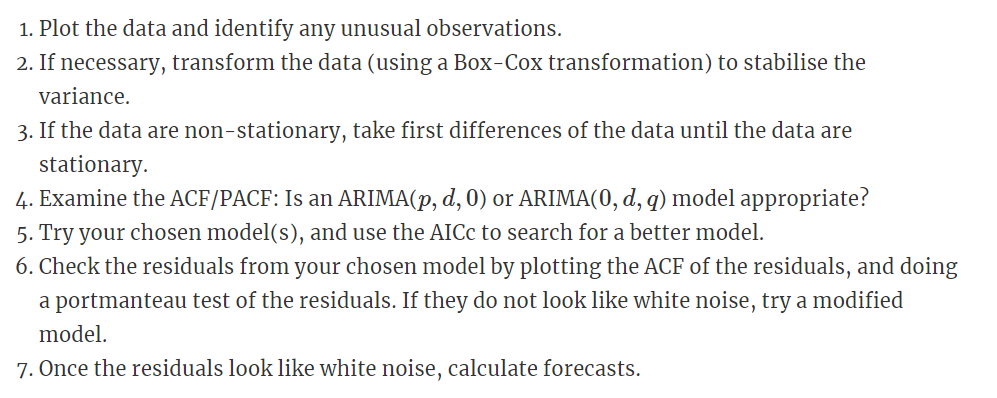
The Hyndman-Khandakar algorithm only takes care of steps 3–5.

ARIMA

Applications of Data Science - Class 21

Giora Simchoni

gsimchoni@gmail.com and add #dsapps in subject

Stat. and OR Department, TAU

2023-04-10

Motivation

Random Processes & Stationarity

White Noise

Random Walk

Simple Moving Average

Stationarity

How to “make” Random Walk stationary?

Autoregessive Processes

AR(p)

AR(1)

AR(1)

AR(1) - ACF

AR(1) - Lag Scatterplots

AR(2)

AR(2)

AR(2) - ACF

Stationarity Conditions

Unit Root Tests

Moving Average Processes

MA(q)

MA(1)

MA(1) - ACF

MA(1) - Lag Scatterplots

MA(1) - Inveritibility

MA(1) - Inveritibility

ARIMA

ARMA(p, q)

ARMA(1, 1)

ARIMA(p, d, q)

Estimation

Least Squares: AR(1)

Least Squares: MA(1)

MLE: AR(1)

MLE: AR(1)

Model Selection

The Old Art of Model Selection

AIC, AICc

ARIMA in fable

ARIMA in fable

ARIMA in fable

Practical Modeling

Forecasting

Seasonal ARIMA

`gsimchoni@gmail.com` and add `#dsapps` in subject

ARIMA in `fable`

ARIMA in `fable`

ARIMA in `fable`